2 Key Points

2.1 Mendelian Errors

Parent and offspring will never be opposing homozygotes (one \(aa\), other \(AA\)) at a locus, except due to genotyping errors. This metric is easy and quick to calculate even in very large datasets, and provides a good way to subset candidate parents (done by sequoia internally), or to check if an existing pedigree is consistent with new genetic data (function CalcOHLLR(, CalcLLR=FALSE)).

The count of opposing homozygous (OH) SNPs is not always a reliable indicator to distinguish parents from not-parents. When the genotyping error rate is high, true parent–offspring pairs may have a high OH count, while some full siblings and other close relatives may have a very low OH count. Therefore, sequoia() uses OH only as a filter to reduce the number of candidate parents for each individual, and uses likelihood ratios for actual assignments.

2.1.1 Parent-pairs

The number of Mendelian errors in an offspring-mother-father trio includes the OH counts between offspring and each parent, as well as cases where the offspring should have been heterozygous, but isn’t (mother \(aa\), father \(AA\), offspring \(aa\) or \(AA\)), and cases where it is heterozygous, but shouldn’t be (when mother and father are identical homozyotes). This metric is used to subset ‘compatible’ parent-pairs when there are candidate parents from both sexes, or with unknown sex.

2.1.2 Maximum mismatches

The maximum number of Mendelian mismatches, and mismatches between potential duplicates, is from version 2.0 onward calculated by CalcMaxMismatch(), based on the (average) genotyping error rate. This parameter can no longer be altered directly, but can be changed via parameters Err and ErrFlavour.

2.2 Likelihoods

Assignments are based on the likelihods for all different possible relationships between a pair, calculated conditional on all assignments made up onto that point. If the focal relationship is more likely than all alternatives (by a margin Tassign), the assignment is made.

The relationships are condensed into seven categories (Table 2.1). Under the default settings (Complx='full'), these also include their combinations (section Unusual relationships), e.g. a pair may be both paternal half-siblings and maternal aunt/niece if they were produced by a mother-daughter pair mating with the same male.

Table 2.1: Main relationships considered
	Relationship
PO	Parent - offspring
FS	Full siblings
HS	Half siblings
GP	Grandparental
FA	Full avuncular (aunt/uncle)
HA	Half avuncular (+ other 3rd degree)
U	Unrelated

To reduce computational time, these likelihoods are only calculated after filtering pairs based on the number of Mendelian errors, their age difference, and a quick calculation of LLR(focal / unrelated) without conditioning on any earlier assigned relatives (must pass Tfilter).

For any pair of genotyped individuals, these seven likelihoods can be calculated with CalcPairLL().

2.3 Genotyping errors

2.3.1 Effect

A higher rate of genotyping errors leads to more false negatives and more false positives during pedigree reconstruction, as illustrated in Figure 2.1. The magnitude of the effect varies: One wrong assignment due to a few genotyping errors in a key individual may have numerous knock-on effects, while dozens of genotyping errors in ‘dead end’ individuals may have no consequences at all.

The simulations (SimGeno()) assume amongst others that genotyping errors are independent from each other and from a sample’s call rate, and likely give a more optimistic picture than real data.

2.3.2 Assumed genotyping error rate `Err`

The reduced performance at high genotyping error rates can be somewhat mitigated by running sequoia() with a roughly correct presumed genotyping error rate Err (Figure 2.1: compare red vs yellow symbols at an error rate of 1-2%).

Among others, when Err is much lower than the actual genotyping error rate, some true parent-offspring pairs will be assigned as full siblings. On the other hand, when Err is much higher than the actual genotyping error rate some true full siblings may be classified as parent-offspring, potentially leading to various ‘secondary’ errors. This trade-off can be explored using CalcPairLL() if some known parent-offspring and full sibling pairs are available.

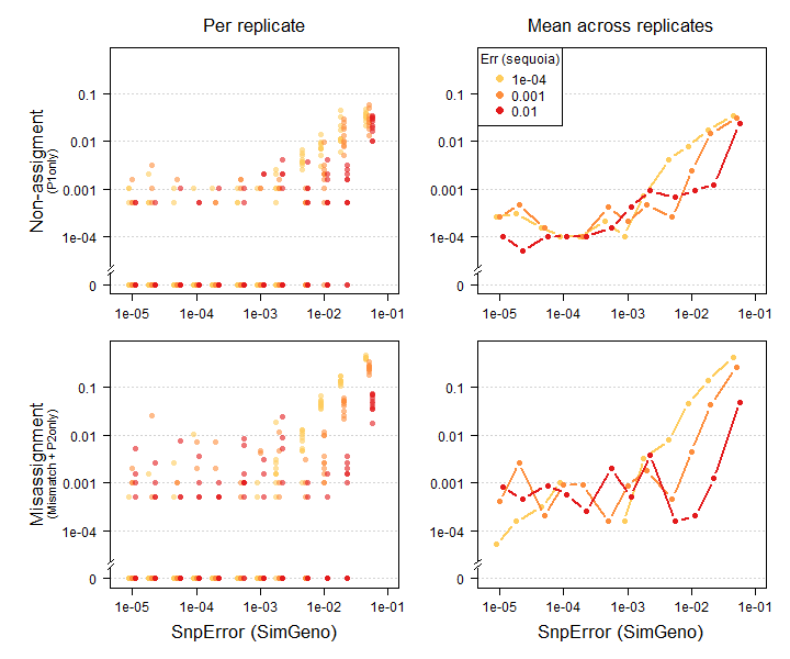
High simulated genotyping error rate (x-axes) increases both false negatives (top) and false positives (bottom). A roughly correct presumed error rate (colours) improves performance. Results from pedigree Ped_HSg5 with 200 SNPs, call rate 0.99, 40% of parents non-genotyped. Diamonds: means across 10 replicates.

Figure 2.1: High simulated genotyping error rate (x-axes) increases both false negatives (top) and false positives (bottom). A roughly correct presumed error rate (colours) improves performance. Results from pedigree Ped_HSg5 with 200 SNPs, call rate 0.99, 40% of parents non-genotyped. Diamonds: means across 10 replicates.

NOTE that the default assumed genotyping error rate of 0.01% is based on data from a SNP array after stringent quality control; in many cases the genotyping error rate will be (much) higher ¹. It is typically worthwhile to explore if and how results change when you vary this parameter, possibly in combination with non-default values for the thresholds Tfilter and Tassign. Do keep in mind the relative consequences of potential misassignments (false positives) versus non-assignments (false negatives) during later use of the pedigree.

2.3.3 Performance with high genotyping error rates

sequoia does not cope well with high rates of genotyping errors, as the sequential approach (see Background) can lead to a cascading avalanche of assignment errors. If the rate is around 1%, be cautious when interpreting the results and please use EstConf() to estimate the assignment error. With genotyping error rates above 5% I would strongly suggest to use MCMC-based approaches, or other approaches more robust to poor genotyping quality.

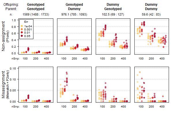
Non-assignment (top) and assignment errors (bottom) for a range of SNP numbers (x-axes) and simulated genotyping errors (colours). sequoia presumed error rates (‘Err’) set equal to simulated error rates. Results for a deer pedigree with overlapping generations and inbreeding; 40% of parents were presumed non-genotyped, call rate=0.99 for remainder.

Figure 2.2: Non-assignment (top) and assignment errors (bottom) for a range of SNP numbers (x-axes) and simulated genotyping errors (colours). sequoia presumed error rates (‘Err’) set equal to simulated error rates. Results for a deer pedigree with overlapping generations and inbreeding; 40% of parents were presumed non-genotyped, call rate=0.99 for remainder.

Assignment of genotyped parents to genotyped offspring is fairly robust to low SNP number and high genotyping errors (left-most column in Figure 2.2), while pedigree links involving a dummy individual are more prone to mis-assignment and non-assignment (columns 2-4 in Figure 2.2). In these simulations, all SNPs are completely independent, call rate is high, and founders are unrelated; in real data the overall performance is probably lower but the patterns will be similar.

2.3.4 Effect on runtime

Computational time tends to increases with both simulated and assumed genotyping error rate, as the time-saving filtering steps become less effective (Figure 2.3).

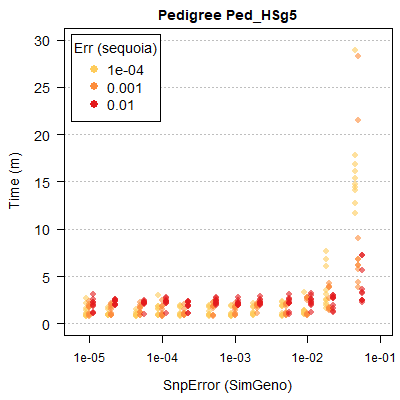
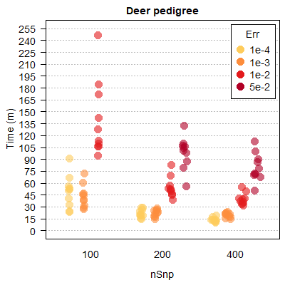
Figure 2.3: Runtimes are shorter with lower genotyping error rates and more SNPs

2.3.5 Error matrix

Different genotyping methods are likely to have different error structures (Table 2.2). Therefore, from version 2.0 sequoia allows fine-scale control over how potential genotyping errors are accounted for. An error matrix with the probability to observe genotype \(G\) (columns), conditional on actual genotype \(g\) (rows), can now be specified via parameter ErrFlavour. The current default (version2.0) is given in Table 2.2, and previous defaults are shown in the help file of ErrToM(). The slight differences between versions only have any consequences when the error rate is high (\(>1%\)).

Table 2.2: Probability of observed genotype (columns) conditional on actual genotype (rows) and per-locus error rate E
	aa	Aa	AA
aa	\((1-E/2)^2\)	\(E\times(1-E/2)\)	\((E/2)^2\)
Aa	\(E/2\)	\(1-E\)	\(E/2\)
AA	\((E/2)^2\)	\(E\times(1-E/2)\)	\((1-E/2)^2\)

From version 2.7 onwards, it is also possible to specify the genotyping error structure as a length 3 vector, with probabilities (between brackets = current defaults):

hom|hom: an actual homozygote is observed as the other homozygote (\((E/2)^2\))
het|hom: an actual homozygote is observed as heterozygote (\(E\\times(1-E/2)\))
hom|het: an actual heterozygote is observed as homozygote (\(E/2\))

During pedigree inference, the error rate is presumed equal across all SNPs. It is also assumed that none of the errors (or missingness) are due to heritable mutations.

2.3.6 Estimate

Function SnpStats() can estimate the genotyping error rate per SNP, conditional on a provided pedigree and error structure (ErrFlavour). These estimated error rates will not be as accurate as from duplicate samples, since a single error in an individual with many offspring will be counted many times, while errors in individuals without parents or offspring will not be counted at all.

2.4 Birth years & Ageprior

For details, including worked examples, mathematical framework, and full range of options, please see the age vignette.

Providing individual birth years will typically greatly improve the completeness and speed of pedigree reconstruction. Age data is used to subset the potential relationships between each pair, and is required to orientate parent–offspring pairs the right way around. Birth year information is not strictly required for every individual: parent-parent-offspring trios can be assigned even in absence of any age data, as long as the sex of either parent is known.

‘Birth year’ should be interpreted loosely, as the time unit (week/month/year/decade/…) of birth/hatching/germination/… .

For individuals (or ‘mystery samples’) with unknown birth years, the probability that they were born in year \(y\) can be estimated using CalcBYprobs(). This relies on the (estimated) birth years of their parents and offspring, and the age distribution of parent-offspring pairs as specified in the age prior.

2.4.1 Definition & interpretation

The ‘agepriors’ as used by sequoia() is not an official term, nor a proper prior, but a set of age-difference based probability ratios which can be interpreted as

If I were to pick two individuals with an age difference \(A\), and two individuals at random, how much more likely are the first pair to have relationship \(R\), compared to the second pair?

The value may vary from \(0\) (impossible), to \(1\) (just as likely), and typically not far beyond \(10\) (10x as likely). This quantification allows age differences to be used jointly with genetic information, which is mostly done in a conservative fashion (except when UseAge='extra'): only when the focal relationship is the most likely both when considering only genetic data, and when considering genetic + age data, is the assignment made. ‘Most likely’ applies to from the set of possible relationships, i.e. those with an age prior value \(>0\).

For example, in datasets with only one or two ageclasses, it is worth contemplating whether or not avuncular relationships should be considered as alternatives to siblings. The behaviour can be changed by explicitly declaring generations as Discrete (avuncular cannot have age difference of 0), and/or by setting MaxAgeParent.

You can find extensive details about the ageprior in this separate vignette, including worked examples, mathematical framework, and full range of options.

2.4.2 Implementation

Parentage assignment is run with an ageprior only specifying that parents and offspring cannot be the same age. The resulting ‘scaffold pedigree’ is then used by MakeAgeprior() to estimate the dataset-specific age-difference distributions for each relationship (mother, father, full sibling, maternal and paternal half sibling), which are standardised by the age-difference distribution among all pairs. The resulting ageprior probability ratios are then used during full pedigree reconstruction (Figure 2.4).

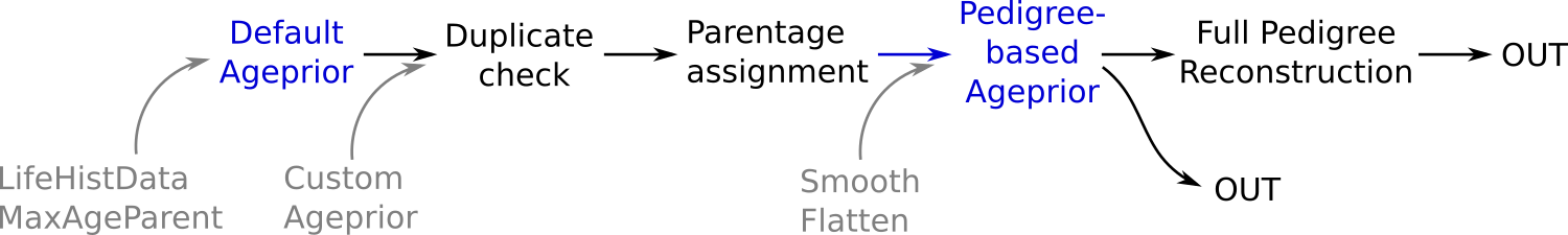
Figure 2.4: Ageprior pipeline overview

When running sequoia(), arguments can be passed to MakeAgePrior() via args.AP.

2.4.3 Smooth & Flatten

Often not all biologically possible age-differences are present in the scaffold pedigree. Therefore MakeAgeprior() by default applies a correction to allow for relatives to differ 1-2 years more in age than observed in its input pedigree, and to smooth out any dips or gaps in the age distributions. However, when such abrupt terminations or gaps are biologically meaningful, these corrections can and should be turned off (Smooth=FALSE and/or Flatten=FALSE). This is done automatically in case discrete generations are declared (Discrete=TRUE) or detected in the scaffold pedigree.

2.4.4 Age-based non-assignment

Any genetically identified parent-offspring pairs and other relatives which are deemed impossible based on their age difference and the age prior matrix, and thus not assigned, can be found by GetMaybeRel(). You may then correct or discard their birth years and/or update the ageprior to allow for their age difference (see Customising the ageprior), and re-run pedigree reconstruction.

2.5 Parent LLR

When parentage assignment or pedigree reconstruction is completed (when the total likelihood has asymptoted), a log10-likelihood ratio (LLR) is calculated for each assigned parent-offspring pair. This is

The ratio between the likelihood of being parent and offspring, versus the next-most-likely relationship between them, conditional on all other relationships in the pedigree.

This differs from for example Cervus (Marshall et al. 1998), which returns the ratio between the likelihood that the assigned parent is the parent, versus that the next most likely candidate is the parent.

The LLRs for the dam and sire separately are calculated by temporarily dropping the co-parent (if any), and calculating the likelihoods assuming the co-parent is a random draw from the population. The LLR for the parent-pair is the minimum of the dam and sire LLR, each conditional on the co-parent. To retrieve the likelihoods underlying each ratio, use CalcPairLL(); specify column dropPar1 for single-parent likelihoods.

Since this step can be quite time-consuming, sequoia() can be run with CalcLLR=FALSE, and CalcOHLLR() can be run separately later. That function can also calculate parental LLR’s for any existing pedigree, including for any non-genotyped individuals with at least one genotyped offspring.

2.6 Confidence

The parental likelihood ratio does not necessarily indicate how likely it is that the assignment is correct. Pedigree-wide confidence probabilities can, among others, be estimated as follows

Simulate genotype data according to the reconstructed (or an existing) pedigree, imposing realistic levels of missingness and genotyping errors (SimGeno());
Reconstruct a pedigree from the simulated data (sequoia());
Count the number of mismatches between the ‘true’ (input) pedigree and the pedigree reconstructed from the simulated data (PedCompare()).

When repeated at least 10–20 times, the proportion of assignments that is correct then provides an estimate of the confidence probability. This will be an optimistic estimate, as SimGeno() assumes all SNPs are independent, that parental genotypes are missing at random, and makes various other simplifying assumptions.

This process is conveniently wrapped in the function EstConf(), which calculates separate confidence levels for dams and sires (which may have very different sampling proportions), for genotyped and dummy parents, and for single parents and members of parent-pairs. The process can be rather time consuming, but from version 2.1 onwards it is possible to run on multiple computer cores in parallel.

2.7 Low assignment rate

Pedigree reconstruction with sequoia() regularly suffers from a low assignment rate, especially when only a small proportion of parents have been genotyped. This is fundamental to the method: when in doubt, MCMC approaches will return an assignment with a low posterior probability, but sequoia() will return no assignment at all.

In sequoia(), an incorrect assignment early on may cause a cascade of other incorrect assignments later in the run, and great care is taken to prevent this. On the flip side, when there is limited genetic or birth year information and/or very few parents have been genotyped, the cascade of correct assignments, where maternal assignments fascilitate paternal assignments and v.v. (Figure 2.5), may never take off. For such situations, different programs with MCMC based approaches are more suitable.

Figure 2.5: Sibship clustering of individuals A-D

2.7.1 Causes

There are four main causes a pair of true relatives are not assigned, which are not mutually exclusive:

There is more than one type of relationship possible between the pair, which cannot be distinguished with certainty (details below);
The type of relationship is clear (e.g. half siblings), but it is unclear whether they are maternal or paternal relatives;
It is clear the pair are mother and daughter (or grandmother – grand-granddaughter), but it is unclear which of the two is the (grand)mother, due to unknown birth year(s) and absence of a ‘complementary’ candidate father (and analogous for father-son);
There is more than one plausible candidate (dummy) (grand)parents of one sex, all of which are more likely to be a parent than otherwise related, even when considered jointly. This includes the situation where true offspring are among the candidate parents due to unknown birth years.

For more details, see FAQ.

Cause (1) has two common underlying causes, which again are not mutually exclusive:

1a. Half-siblings, grandparent–grand-offspring and full avuncular pairs are genetically indistinguishable, even with perfect genetic data. Assignment of half-sibling pairs is only possible when grand-parental and avuncular relationships can be excluded based on the age-difference of the pair, or when both individuals already have a parent assigned (in which case the likelihoods do differ). 1b. The SNP data is not informative enough to clearly distinguishing between parents and full siblings, between full and half siblings, between half siblings and cousins, etc.. The problem may be specific to a few pairs and due to the randomness of Mendelian segregation, or be widespread due to a low number of SNPs, low MAF, and/or high error rate.

2.7.2 Remedies

Sometimes it is possible to reduce the number of non-assigned parents in the pedigree by providing more life history data, removing SNPs with the highest error rates, or lowering the thresholds Tfilter and/or Tassign. The latter will reduce the probability of false negatives, but at the same time increase the probability for false positives. If inbreeding and double relationships are rare, using Complx='simp' may also improve assignment (see here).

Small adjustments may ‘get the snowball rolling’ (Figure 2.5) and greatly increase assignments. Once a sibling pair is assigned, adding additional siblings to the cluster becomes progressively easier as it becomes more and more obvious whether an individual is related to all individuals in the sibship, or to none.

There are functions in the package that may help identify whether there are un-assigned likely relatives in the dataset, and/or the probable cause of non-assignment of presumed relatives:

GetMaybeRel() will identify any pairs that are likely to be 1st or 2nd degree relatives. It can do so as-is, or conditional on a (reconstructed) pedigree. It may also provide clues whether this is e.g. due to unknown birth years or an impossibility to tell the different 2nd degree relationships apart (TopRel = ‘2nd’).
CalcPairLL() will return for a specified set of pairs the likelihoods to be parent-offspring, sibling, … (Table 2.1). The pairs may be the output from GetMaybeRel(), or e.g. pairs of litter mates. This may e.g. show that it is unclear whether the pair are full or half siblings, but they are probably either one or those. Or it may show the pair are probably either half-siblings or 3rd degree relatives (half-avuncular, cousins, great-grandparent). The latter may be ‘declared’ half-siblings if the breeding scheme or field data (e.g. being litter mates) makes 3rd degree relatives highly unlikely. You can specify a pedigree and/or ageprior to condition on, and can include a pair multiple times with different age difference or focal relationship to explore their effects on the likelihoods and thereby the LLR.
use of mitochondrial haplotype sharing data to distinguish between maternal and paternal relatives. See the mtDNA vignette for details.

References

Marshall, T C, J B K E Slate, L E B Kruuk, and J M Pemberton. 1998. “Statistical Confidence for Likelihood-Based Paternity Inference in Natural Populations.” Molecular Ecology 7 (5): 639–55.

but changing the default value is likely to cause problems for people re-using old code.↩︎