6 Small sample correction
6.1
Calculating the proportion of pairs with relationship \(R\) and age difference \(A\) in a pedigree is reasonably straightforward, but generating a matrix that is useful for subsequent pedigree reconstruction under a wide range of ‘non-ideal’ situations is not.
6.2 The problem
A major challenge is that when an age/relationship combination is not observed in the input pedigree, its ageprior value will be \(0\), and without correction that age/relationship combination will be deemed impossible during full pedigree reconstruction. For example, if mother-offspring pairs with age differences of 1, 2, 3, and 5 years are observed, it would infer that females never breed at age 4. This seems highly unlikely from a biological perspective, and is much more likely a sampling artefact. This does matter during full pedigree reconstruction: if the true maternal grandmother is 8 years older than one of her grandchildren, she would not be assigned, because mothers cannot be age 4.
As another example, imagine that no candidate fathers at all were sampled. Based on the parentage-only scaffold pedigree, the counts in the father column of tblA.R would be \(0\) for all age differences. Consequently, all age differences would be disallowed for father-offspring pairs during subsequent full pedigree reconstruction, including for dummy fathers, and no paternal sibships would be clustered.
Incorrect agepriors can also lead to false positives: when it is wrongly believed the age difference of a genetic half-sib pair makes it impossible for them to be maternal siblings, they will likely be assigned as paternal half-siblings. More individuals may then be added to this erroneous paternal sibship, potentially setting off a snowball effect of wrong assignments.
To minimise these problems, MakeAgePrior() applies two generic, one-size-fits-most corrections: a Smoothing of dips and padding of the tails, and a Flattening approach whereby a weighed average of the pedigree-based and flat default ageprior is taken (Figure 6.1).
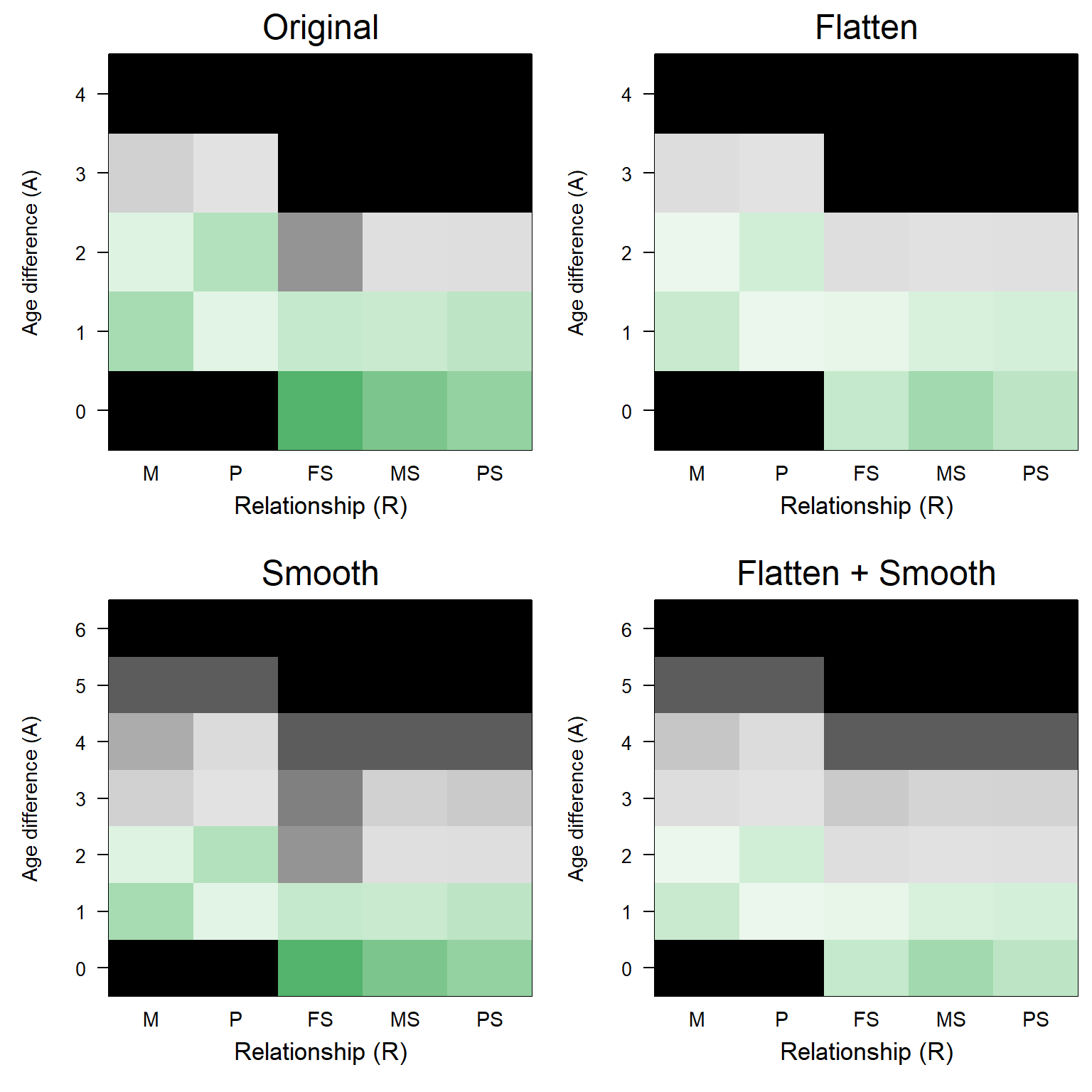
Figure 6.1: Smoothed & Flattened agepriors for overlapping generations (griffin example). Note the different y-axes; non-displayed age differences have an ageprior of zero for all R.
6.3 Smooth
When Smooth=TRUE, the tails of the distributions are ‘stretched’ and any dips are smoothed over. It defaults to TRUE, as there is only rarely a detrimental effect of smoothing when none is required. Exception is when generations are discrete; when this is detected or declared by the user, Smooth is set to FALSE automatically.
A ‘dip’ is defined as a value that is less than 10% of the average of its neighbouring values (age differences of one year less/more), and both neighbours have values \(>0\). It is then changed to the average of the two neighbours. Peaks are not smoothed out, as these are less likely to cause problems than dips, and are more likely to be genuine characteristics of the species.
The front & end tails of the distribution are altered as follows:
SmoothAP <- function(V, MinP) {
  Front <- max(1, min(which(V > MinP)), na.rm=TRUE)
  End <- min(max(which(V > MinP)), length(V), na.rm=TRUE)
  if (Front > 1 & V[Front] > 3*MinP)    V[Front -1] <- MinP
  if (End < length(V))                                V[End +1] <- V[End]/2
  if ((End+1) < length(V) & V[End+1] > 3*MinP)  V[End+2] <- MinP
  # ... dip-fixing ...
  V
}

LR.RU.A <- apply(LR.RU.A, 2, SmoothAP, MinP = 0.001)
There is no way to change the behaviour of Smooth, except turning it on or off. If for example a longer tail is required at either end, or more thorough smoothing is needed, you will need to edit the ageprior matrix yourself (see Customisation).
6.4 Flatten
The ageprior is ‘flattened’ by taking a weighed average between the ageprior based on the pedigree and birth years, and a flat default ageprior based on the maximum age of parents only (user-specified, pedigree-estimated, or maximum age difference in LifeHistData):
AP.pedigree <- MakeAgePrior(Ped_griffin, Smooth=FALSE, Flatten=FALSE,
                            quiet=TRUE, Plot=FALSE)
AP.default <- MakeAgePrior(MaxAgeParent = 3, quiet=TRUE, Plot=FALSE)

knitr::kable(list(AP.pedigree, AP.default),
             caption = "Pedigree-based ageprior (left) and default, flat ageprior (right).",
             booktabs=TRUE)
|
|
\[\begin{equation} \alpha*_{A,R} = W_R \times \frac{P(A|R, \text{sampled})}{P(A, \text{sampled})} + (1-W_R) \times I_{A,R} \end{equation}\]
where \(W_R\) is a weight based on \(N_{R}\), the number of pairs with relationship \(R\) and known age difference. \(I_{A,R}\) is an indicator whether the age-relationship combination is possible (1) or not (0) based on the maximum parental age (i.e., the flat default ageprior). \(\alpha_{A,R} = P(A|R, \text{sampled}) / P(A, \text{sampled})\) is the raw pedigree-based ageprior.
AP.flattened <- MakeAgePrior(Ped_griffin, Smooth=FALSE, Flatten=TRUE, quiet=TRUE, Plot=FALSE)| M | P | FS | MS | PS | |
|---|---|---|---|---|---|
| 0 | 0.000 | 0.000 | 2.761 | 3.574 | 2.918 |
| 1 | 2.698 | 1.655 | 1.783 | 2.270 | 2.321 |
| 2 | 1.693 | 2.467 | 0.598 | 0.760 | 0.721 |
| 3 | 0.548 | 0.972 | 0.000 | 0.000 | 0.000 |
| 4 | 0.000 | 0.000 | 0.000 | 0.000 | 0.000 |
6.4.1 Weighing factor & lambdaNW
The weighing factor \(W_R\) follows a asymptotic curve when plotted against sample size (Figure 6.2), and is calculated as \[\begin{equation} W_R = 1 - \exp(-\lambda_{N,W} * N_R) \text{ .} \end{equation}\]
By default \(\lambda_{N,W}=-\log(0.5)/100\) (input parameter lambdaNW), which corresponds to \(W_R< 0.5\) if \(N_R < 100\); i.e. if there are fewer than 100 pairs with known age difference, the flat ageprior weighs heavier than the pedigree-inferred ageprior, and the opposite if there are more than 100 pairs. When \(\lambda_{N,W}\) is large (say \(>0.2\)), Flatten is effectively only applied for relationships with very small sample size (e.g. \(W=0.86\) at \(N=10\)), while when \(\lambda_{N,W}\) is small (say \(<0.0001\)) there is effectively no contribution of the pedigree even with very large sample size (e.g. \(W=0.10\) at \(N=1000\)).
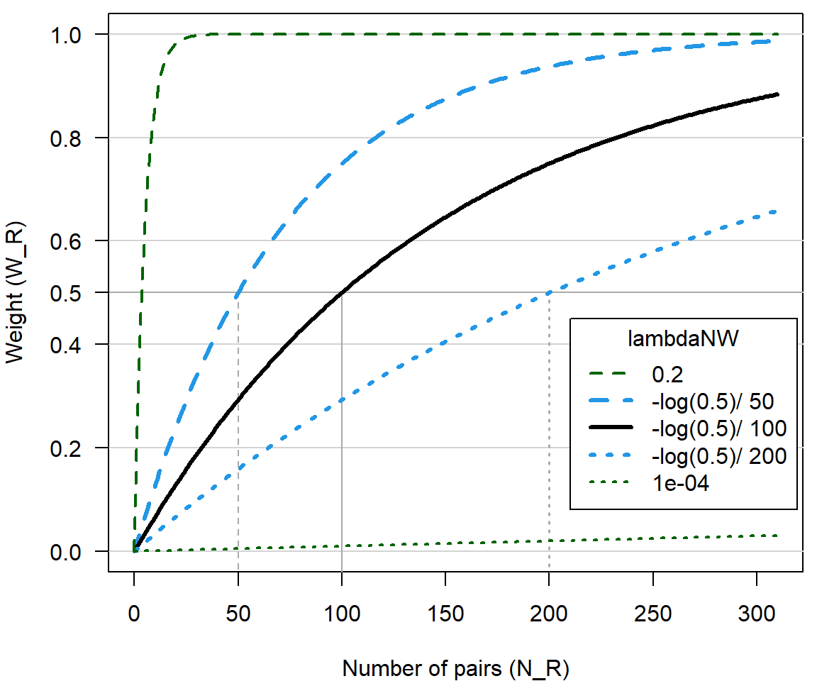
Figure 6.2: Weights versus number of pairs with relationship R, for weighed average between pedigree-derived ageprior and flat 0/1 ageprior
Since the number of pairs with known age difference will differ between relationship types, so will the weights:
AP.griffin$Weights## M P FS MS PS
## 0.6857 0.6769 0.0341 0.7762 0.6701By chance there are more maternal than paternal sibling pairs in this pedigree, due to one large maternal sibship (see SummarySeq(Ped_griffin)), and thus the weight for ‘MS’ is larger than for ‘PS’. We can use the pair counts per relationship to double check the weights:
NAK.R # counts per relationship (column sums of tblA.R)## M P FS MS PS X
## 167 163 5 216 160 19900lambdaNW <- -log(0.5)/100 # default input value
W.R <- 1 - exp(-lambdaNW * NAK.R[1:5])
round(W.R, 4)## M P FS MS PS
## 0.6857 0.6769 0.0341 0.7762 0.67016.4.2 Sample size vs. sampling probability
In theory, the sampling probability per relationship could be estimated, and used to calculate some correction factor for equation (2.2). In practice, this requires some strong assumptions about the number of assignable parents (i.e. distinction between pedigree founders and non-founders) and the number of sibling pairs (i.e. distribution of sibship sizes). Moreover, this correction factor would depend on the total number of sampled individuals in a non-nonsensical way: removing individuals without assigned parents from the pedigree would ‘magically’ increase our faith in the ageprior estimated from the remainder of the pedigree. Therefore, the degree of correction by Flatten depends only on the number of individual pairs per relationship with known age difference, not on a proportion.